Dimuons Revisited#
We will now reconstruct the mass of the Z boson using dimuon events, applying a more careful and systematic approach based on the techniques we have learned so far. We begin my importing all of the libraries we need, as well as re-loading the muon data we previously downloaded.
# Import all neccesary libraries
import numpy as np
import uproot
import awkward as ak

import hist
import matplotlib.pyplot as plt
import mplhep as hep
hep.style.use("CMS") # use CMS style for plots
file = uproot.open(
    "./uproot-tutorial-file.root"
)
tree = file["Events"]
muons = tree.arrays()
muons
For future convenience, we will re-organize the branches of the loaded data to something a bit more intuitive. First, we will have each muon in an event correspond to an Awkard record (recall: the equivalent to a dictionary) with all of the particle’s properties. We will also rename the observables to something less redundant, since we know we are dealing only with muon data. We can achieve this by using the ak.zip function.
muons = ak.zip(
    {
        "pt": muons["Muon_pt"],
        "eta": muons["Muon_eta"],
        "phi": muons["Muon_phi"],
        "charge": muons["Muon_charge"]
    }
)
muons
Before continuing, keep in mind that the process of interest is the decay of the \(Z\) into a pair of leptons. The Feynman diagram for this can be seen below.
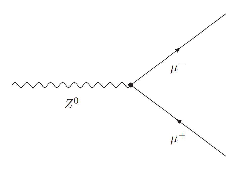
Fig. 8 \(Z\to\mu\mu\) Feynman diagram#
Since we don’t know where the muons originated from and whether or not it came from the decay of a \(Z\), we will find all possible combinations of two muons in each event. For this we use ak.combinations(). One of the convenient things with this function is that if there is less than 2 muons in an event, and thus its impossible to make a combination of two muons, the array of pairs for that event is empty (i.e. its “filtered” out).
pairs = ak.combinations(muons, 2)
pairs
Now we separate each pair of muons into their own arrays. This will simplify the desired computations later on and make the code readable.
mu1, mu2 = ak.unzip(pairs)
Let’s now use the mass formula we used before to compute the dimuon mass.
m_dimuon = np.sqrt(
    2 * mu1["pt"] * mu2["pt"] * (np.cosh(mu1["eta"] - mu2["eta"]) - np.cos(mu1["phi"] - mu2["phi"]))
)
m_dimuon
We now want to plot these mass values in a histogram. However, you can’t plot a jagged array directly. You must first use a function such as ak.ravel() to “unravel” the array into a flat array. We then pass that into a hist.Hist object and plot it using Matplotlib.
fig, ax = plt.subplots()

h = hist.Hist(hist.axis.Regular(120, 0, 120, label="mass [GeV]"))
h.fill(ak.ravel(m_dimuon))

h.plot1d(ax=ax, histtype="step", color="red", linewidth=0.75, label="$m_{\mu\mu}$")
ax.set_title("Dimuon Mass")
ax.set_ylabel("Count")
ax.set_xlabel("Mass (GeV)")
ax.legend()

plt.show()
Uh-oh. We seem to have made things worse! The Z peak now looks very small compared to what we obtained before. In order to fix this, we can take into account certain physical considerations which may allow us to reject more of the background. Here are some things to consider:
The highest dimuon mass is more likely to have come from the direct decay of a heavy particle like the Z rather than from lower mass background processes.
The Z boson is electrically neutral so the muons must be of opposite charge in order for there to be charge conservation.
Due to momentum conservation, we expect the muons to not be too far apart in space. (Next chapter!)
Choosing oppositely charged muons#
We first make a mask using mu1 and mu2 that selects muon pairs of opposite charge.
opp_charge_mask = mu1["charge"] + mu2["charge"] == 0
pairs_opposite_charge = pairs[opp_charge_mask]
mu1_opposite, mu2_opposite = ak.unzip(pairs_opposite_charge)
We now compute the mass of these new set of oppositely charged muons.
m_dimuon_opposite = np.sqrt(
    2 * mu1_opposite["pt"] * mu2_opposite["pt"] * (np.cosh(mu1_opposite["eta"] - mu2_opposite["eta"]) - np.cos(mu1_opposite["phi"] - mu2_opposite["phi"]))
)
m_dimuon_opposite
Finally, we plot the masses, making sure to flatten the array.
fig, ax = plt.subplots()

# Making hist
h = hist.Hist(
    hist.axis.Regular(120, 0, 120, label="mass [GeV]")
)

# Filling hist
h.fill(
    ak.ravel(m_dimuon_opposite)
)

# Plotting hist
h.plot1d(ax=ax, histtype="step", color="blue", linewidth=0.75, label=r"$m_{\mu\mu}$ (opposite charge)")
ax.set_title("Dimuon Mass (Opposite Charge)")
ax.set_ylabel("Count")
ax.set_xlabel("Mass (GeV)")
ax.legend()
plt.show()
Choosing highest dimuon mass#
We first get the maximum per-event mass from the computation we did before.
# Highest dimuon mass with opposite charge
max_m_dimuon_opposite = ak.max(m_dimuon_opposite, axis=1)
max_m_dimuon_opposite
The array can’t be used as-is, because it contains None values which we cannot use to fill out histogram. Fortunately, a neat feature of ak.flatten is that it can be used to remove the None values from a flat array.
# ak.flatten is used here to remove None values
max_m_dimuon_opposite = ak.flatten(max_m_dimuon_opposite, axis=0)
max_m_dimuon_opposite
We are now ready to plot!
# Highest dimuon mass with opposite charge plot
fig, ax = plt.subplots()
hist.Hist(
    hist.axis.Regular(120, 0, 120, label="mass [GeV]")
).fill(max_m_dimuon_opposite).plot1d(ax=ax, histtype="step", color="green", linewidth=0.75, label=r"$m_{\mu\mu}$ (max mass, opposite charge)")
ax.set_title("Max Dimuon Mass (Opposite Charge)")
ax.set_ylabel("Count")
ax.set_xlabel("Mass (GeV)")
ax.legend()
plt.show()
Exercise
Instead of maximizing the mass of the dimuon we choose from each event, try selecting the mass closest to the known mass of the \(Z\) boson. (Hint: look up ak.argmin in Google)